Process module: AddRandomUniformPredictors

Process module which adds a random uniform covariate to the dataset. This new covariate can be scaled to an existing covariate.

AddRandomUniformPredictors(.data, name = "RandUnif", scaleTo = NULL)

Arguments

.data

Internal parameter, do not use in the workflow function. .data is a list of a data frame and a raster object returned from occurrence modules and covariate modules respectively. .data is passed automatically in workflow from the occurrence and covariate modules to the process module(s) and should not be passed by the user.

name

Optional argument specifying the name of the new covariate layer. If not specified, it will automatically named.

scaleTo

Optional argument specifying the name of an existing covariate layer which the new random uniform covariate will be scaled to.

Examples

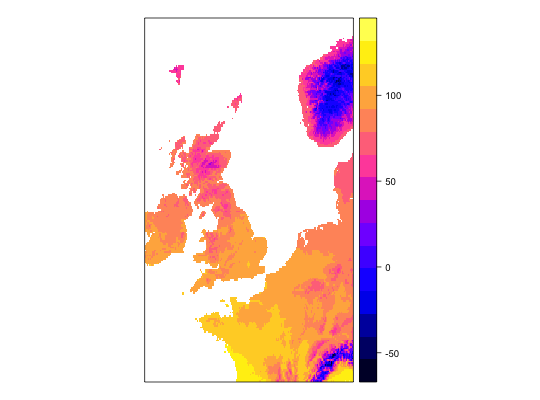
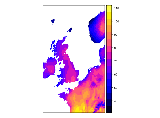
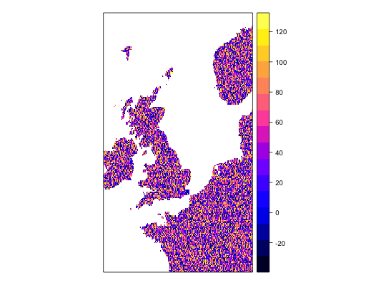
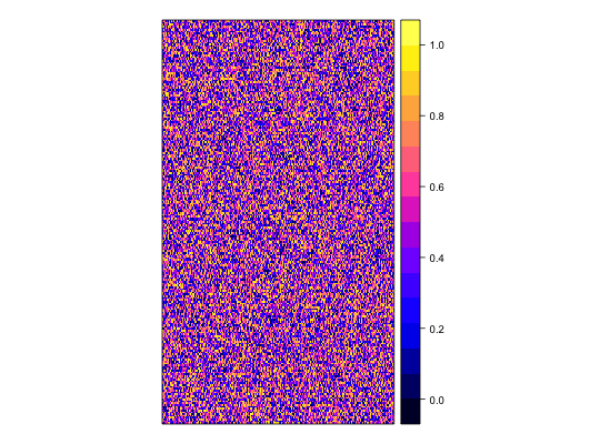
work1 <- workflow(occurrence = UKAnophelesPlumbeus,
   covariate  = UKBioclim,
   process    = Chain(OneHundredBackground,
                   AddRandomUniformPredictors(scaleTo = 'bio1',name = 'Random.bio1'),
                   AddRandomUniformPredictors(scaleTo = 'bio2'),
                   AddRandomUniformPredictors),
   model      = LogisticRegression,
   output     = PerformanceMeasures)
Warning message:
Some extracted covariate values are NA. This may cause issues for some models
Warning message:
You have no cross-validation folds, validation statistics may be misleading
Warning message:
prediction from a rank-deficient fit may be misleading
Warning message:
286 data points removed due to missing data

### Dsiplay resulting covariate maps from each workflow
spplot(work1$process.output[[1]]$ras$bio1)
spplot(work1$process.output[[1]]$ras$bio2)
spplot(work1$process.output[[1]]$ras$Random.bio1.1)
spplot(work1$process.output[[1]]$ras$RandUnif.1)
spplot(work1$process.output[[1]]$ras$RandUnif.2)

### Show resulting model
work1$model.output[[1]]$model$model
#> 
#> Call:  glm(formula = .df$value ~ ., family = "binomial", data = covs)
#> 
#> Coefficients:
#>   (Intercept)           bio1           bio2           bio3           bio4  
#>     -1.342427      -0.534995      -0.472520       0.392092      -0.036863  
#>          bio5           bio6           bio7           bio8           bio9  
#>      0.356548      -0.391765             NA       0.023554      -0.046062  
#>         bio10          bio11          bio12          bio13          bio14  
#>      1.279061      -0.648244      -0.064661      -0.212880       0.248887  
#>         bio15          bio16          bio17          bio18          bio19  
#>     -0.027247       0.223968       0.155035      -0.074517      -0.038476  
#> Random.bio1.1     RandUnif.1     RandUnif.2  
#>      0.007922       0.020959       0.040233  
#> 
#> Degrees of Freedom: 285 Total (i.e. Null);  264 Residual
#> Null Deviance:	    370.2 
#> Residual Deviance: 159.2 	AIC: 203.2
#> 

Author